Interventions for Gang Reduction and Youth Development
The Gang Reduction and Youth Development (GRYD) program in Los Angeles has a program for adolescents at risk of joining gangs. GRYD uses a questionnaire (‘Youth Services Eligibility Tool’, or YSET) to evaluate the eligibility of students for this program. Students are sorted into three categories: low risk, at risk, and high risk. The program aims to provide resources for the at risk group.
The dataset contains the responses of $N \sim 10,000$ students. The questionnaire has $100$ questions, of which only $56$ are used for risk assessment. To calculate risk factor, a student’s score is calculated using nine thematic scales. A student scoring in less than three of the scales is considered to have low risk factor, and a student scoring in more than five of the scales is considered to have high risk factor.
There may be other methods that are more effective at classifying students into three groups. It is important to be able to visualize our data in order to identify features of our dataset and to be able to compare different methods. If each response can be thought of as a point in real coordinate space, we should investigate projecting the space onto two dimensions without loss of information.
Principle Component Analysis
The first method to try is linear dimensionality reduction using Principle Component Analysis (PCA). PCA linearly projects the data onto the directions in which the sample variance is maximized.
Instead of doing analysis directly, I used the graph Laplacian $L$ on either the scales or the questions. Considering that there are nine scales and $56$ questions, a response $x_i \in \mathbb{R}^9$ or $x_i \in \mathbb{R}^{56}$, respectively. The dataset can be written as a graph with nodes $x_i$ and weighted edges $w_{ij}$ corresponding to the similarity in answering the questionnaire. The weights $w_{ij}$ correspond to a Gaussian distribution, scaled according to the Euclidean distance between responses $x_i$ and $x_j$ and a parameter $\sigma$. Then the corresponding graph Laplacian $L = D - W$, where:
\begin{aligned}
W_{ij} &= e^{\frac{-\Vert x_i - x_j \Vert^2}{2\sigma^2}} \\\
D &= \text{diag}\left(\sum_{j=1}^m W_{ij}\right)
\end{aligned}
The graph Laplacian is positive semidefinite, meaning we can decompose it into eigenvalues $\lambda_i \geq 0$ such that $Lv_i = \lambda_i v_i$.
PCA works as follows. Let $\mathbf{V} \subset \mathbb{R}^2$ be the subspace spanned by the basis of the first two unit eigenvectors corresponding to the largest eigenvalues of $L_{d\times d}$, $\lambda_1$ and $\lambda_2$. Then we can project a point $x$ onto $\mathbf{V}$: $$\hat{x} = \text{proj}_\mathbf{V}(x) = \bar{x} + \sum_{i=1}^2 \langle x - \bar{x}, u_i\rangle u_i$$ where $\bar{x}$ is the sample mean. The error using least squares is $$\frac{1}{N} \sum_{n=1}^N \Vert \hat{x_n} - \bar{x}\Vert^2 = \sum_{j=3}^d \lambda_j$$ so the projection minimizes the error by taking the largest two eigenvalues.
Figure 1 shows the results of PCA on the scales. The responses are clearly clustered into three groups, however these three groups do not correspond to Risk Factor (RF). Upon further investigation, they are clustered according to a scale that only has two questions. Thus, this result reflects a property of the questionnaire’s construction which is not meaningful.
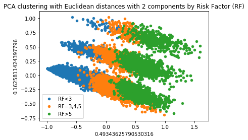
Figure 2 shows the results of PCA on the questions. There is one large cluster with a clear progression from low Risk Factor to high Risk Factor, but there is significant overlap.

Different distance metrics in the weight calculation of the graph Laplacian may yield more desirable results. However, a nonlinear dimensionality reduction approach is far more important.
Nonlinear Dimensionality Reduction
Isomap is a nonlinear dimensionality reduction method that extends metric multidimensional distances (MDS). The algorithm has three steps. First, it performs $k$-nearest neighbors to identify the contour of the manifold. Second, it estimates the geodesic distances by calculating the shortest paths between points. Finally, Isomap performs MDS on the new distance matrix.
Additionally, Isomap is isometric, meaning that the mapping between manifolds preserves distances between points. Since we want to understand how different responses relate to each other, this is crutial. In the 2018 UCLA REU, Yifan Li worked on a methodology for nonlinear dimensionality reduction.
Dynamic Mode Decomposition
In the summer of 2018, I studied the GRYD dataset as a dynamical system using Dynamic Mode Decomposition with Jiazhong Mei and Qinyi Zeng. Please see the report below. In January 2019 I applied the methodology to students who were rejected from the program and analyzed new data from GRYD. We are working on publishing our findings so stay tuned!