Particle Laden Flows
Introduction
A slurry is a mixture of solid particles and liquid. I studied an aspect of slurries called viscous particle laden flow in Dr. Bertozzi’s Applied Math Lab in 2016 and 2017 with other undergraduate students. We used simulations and experiments to study the effects of gravitational and shear forces on bidisperse slurries. I’ve decided to highlight some of our findings on bidensity slurries in this article.
The behavior of these flows are important because they occur in many fields. Mining companies use spiral separators to separate minerals from ore. Mixtures of oil, sand, and water occur in oil spills. Slurries also occur in industrial, biological, and pharmaceutical contexts.

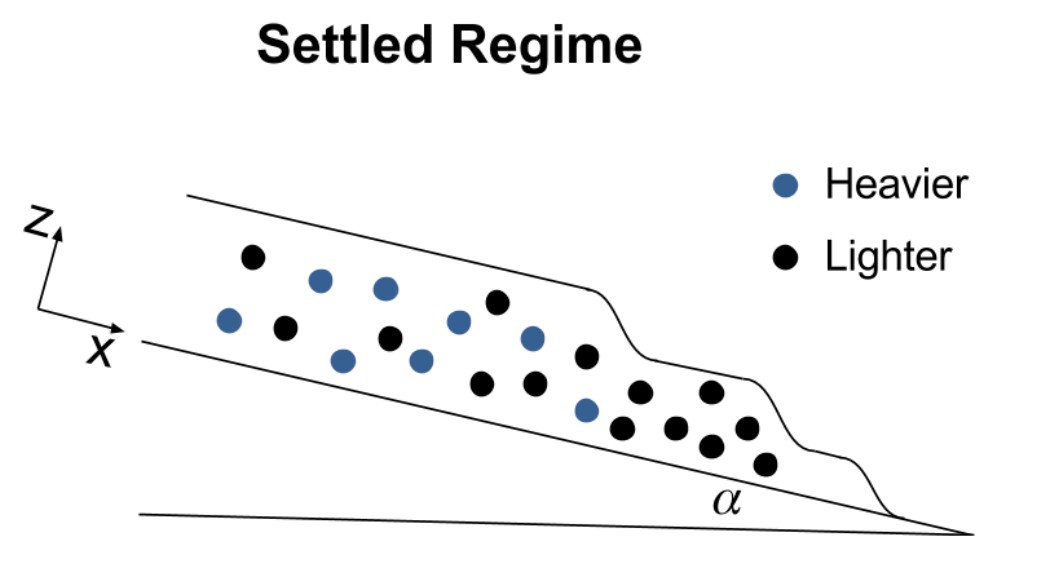
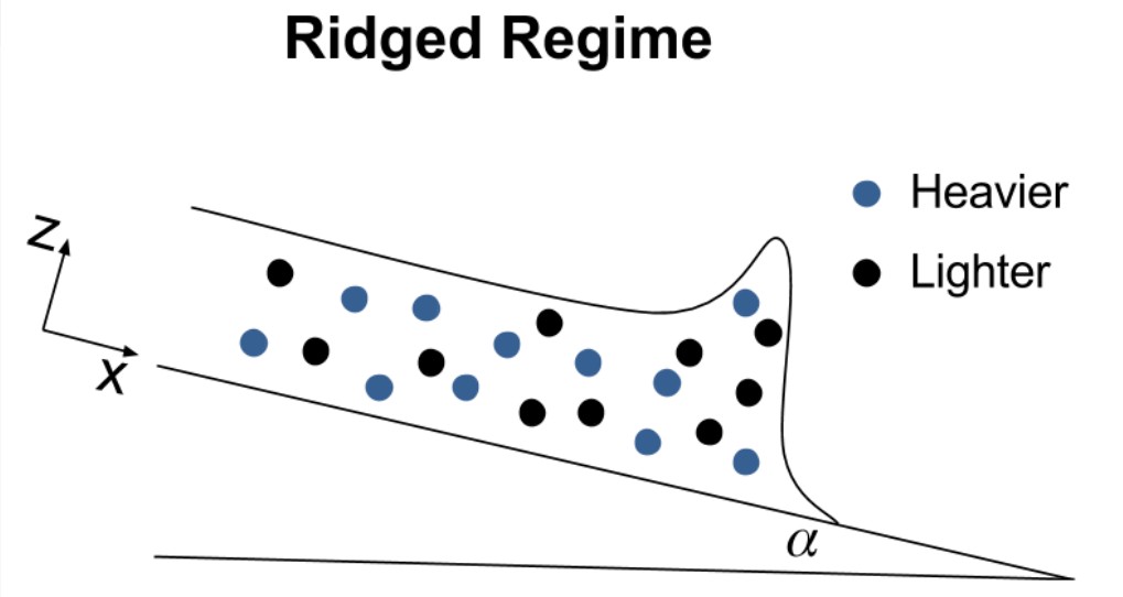
When the mixture flows down a ramp, some interesting behavior occurs. Sometimes the particles separate from the liquid. Sometimes the particles move faster than the liquid, forming a particle-rich ridge at the front of the flow. Sometimes fingers form. We wanted to create a mathematical model to describe the fluid’s dynamics that depends on external forces and the types and quantity of particles present in the slurry.
Previous research123 has developed a force-based model for constant volume monodisperse flow. Lee et. al.4 and Wong and Bertozzi5 extended this model to the bidensity case using experiments and theory, respectively. They used constant volume initial conditions, meaning that a fixed volume of slurry was poured onto the incline and allowed to flow. We adapted their model to use constant flux initial conditions, where the slurry is continuously added to the incline with a constant flow rate. We also performed experiments using the same total volume fraction $\phi_0 = \frac{V_p}{V_t} = 0.4$ parameter, and compared the results to the prediction of the theory.
Theory
Using the Navier-Stokes equation and particle mass conservation, we can create a system of coupled ODEs. Let $\phi_i$, $i=1,2$ to be the volume fraction of particle $i$ to the total volume, $\phi = \phi_1 + \phi_2$, and the $\boldsymbol{J}_i$ term is the flux of particle $i$:
\begin{aligned}
0 &= \nabla \cdot (-pI + \mu(\nabla\boldsymbol{u} + \nabla\boldsymbol{u}^T)) + \rho\boldsymbol{g}. \\\
0 &= \frac{\partial \phi_i}{\partial t} + \boldsymbol{u} \cdot \nabla \phi_i + \nabla \cdot \boldsymbol{J}_i, \quad i=1,2.
\end{aligned}
Assuming equilibrium in the $z$-direction, the resulting system of ODEs relates the dervitives of the shear stress $\sigma$, viscosity $\mu$, and density $\rho$.
To model the height and front position of the fluid and two particles, we introduce depth-averaged particle concentration and volume ratio. Then we have a system of PDEs:
\begin{aligned}
0 &= \frac{\partial h}{\partial t} + \frac{\partial}{\partial x}(h^3f(\bar{\phi},\bar{\chi})) \\\
0 &= \frac{\partial (h\bar{\phi_i})}{\partial x} + \frac{\partial}{\partial x}(h^3g_i(\bar{\phi},\bar{\chi})), \quad i=1,2
\end{aligned}
We consider the Riemann initial condition:
\begin{aligned}
h(x,0) &= \begin{cases} \left[\frac{3\mu(\phi_0)Q}{W\rho(\phi_0)g\sin\alpha}\right]^\frac{1}{3}, & x<0 \
\varepsilon, & x>0 \end{cases} \\\
\bar{\phi}(x,0) &= \begin{cases} \phi_0, & x<0 \
0, \qquad \qquad \qquad ! & x>0 \end{cases} \\\
\bar{\chi}(x,0) &= \begin{cases} \chi_0, & x<0 \
0, \qquad \qquad \qquad ! & x>0 \end{cases} \\\
\end{aligned}
Finally, expressing the system in vector notation we have:
\begin{equation}
U = (h, h\bar{\phi_1},h\bar{\phi_2})^T \\\
F(U) = h^3(f,g_1,g_2)^T
\end{equation}
$$U_t + (F(U))_x = 0$$
We then solve the partial differential equation using an upwind scheme. The height profile can be obtained from $h$ and the particle front profile can be found from plotting the concentration profile.
Experiments
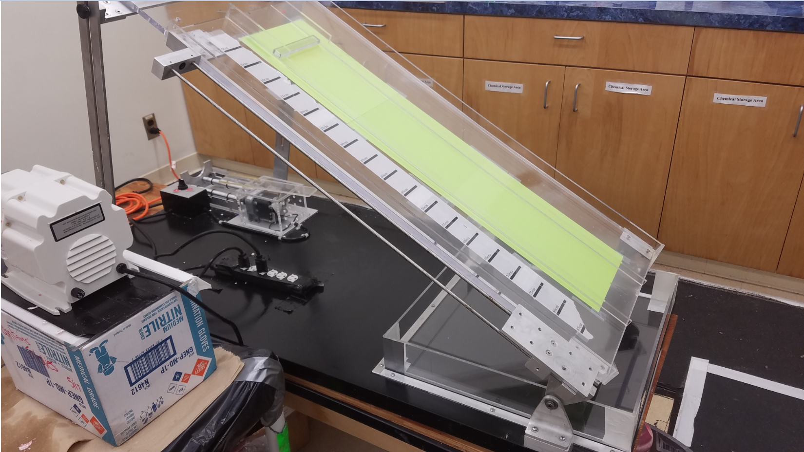
We can perform experiments to track the particle fronts and height profile of the particle laden flow. We can vary the total volume fraction $\phi_0$, the volume ratio between beads $\chi$, and the inclination angle $\alpha$ of the track. In addition, we can have two types of initial conditions: constant volume or constant flux. In the constant volume case we measure and pour a finite volume onto the track. In the constant flux case, we use a pump to continuously add slurry to the track. A picture of the track is below.
In 2017, we used the following materials:
| Particles | density $\rho$ | diameter $d$ | color |
|---|---|---|---|
| Small Glass (P1) | $2.5$ g/cm$^3$ | $0.07-0.125$ mm | pink (dyed) |
| Small Ceramic (P2) | $3.8$ g/cm$^3$ | $0.150-0.180$ mm | blue (dyed) |
| Large Glass (P3) | $2.5$ g/cm$^3$ | $0.40-0.60$ mm | white |
| Large Ceramic (P4) | $3.8$ g/cm$^3$ | $0.40-0.60$ mm | red |
| Fluid | density $\rho$ | viscosity $\nu$ | color |
| PDMS oil | $0.971$ g/cm$^3$ | $10^{-3}$ m$^2$/s | clear |
| The liquid used in all experiments is viscous polydimethylsiloxane (PDMS) oil. For bidensity experiments, we use glass and ceramic beads with the same diameter (P3 and P4). For bidisperse experiments, we use pairs of beads with the same density but different diameters (P1 and P3, or P2 and P4). |
We film the slurry as it flows down the track to capture front position and velocity information. Using MATLAB, we can analyze the concentrations of particles present in different segments of the flow. We identify the front position of each species of particle and the PDMS.
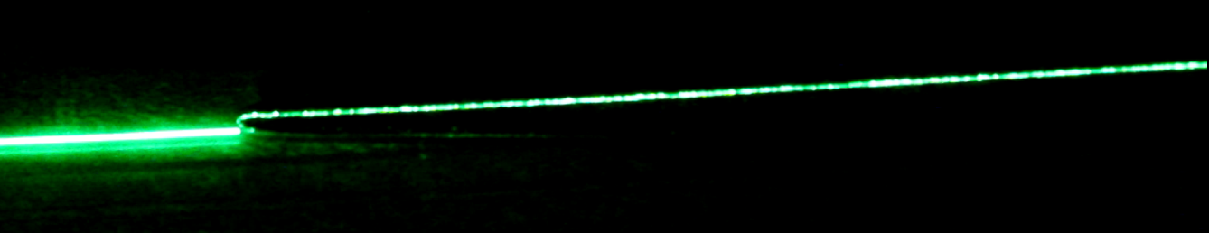
To create a height profile of the flow, we use a laser sheet and analyze video in MATLAB. As shown in Figure 4, the laser line position in the video is distorted by the slurry.
Experimental Results
The constant flux bidensity experiments from 2017 are summarized in Figure 5. As the phase diagram shows, we experimentally see the ridged regime at trials displayed by the blue diamonds, the settled regime at trials displayed by black circles, and the well-mixed regime at trials displayed by red circles.The darker shaded region on the table shows where we expect to see more ridged regimes, and the white area is where we expect to see settled regimes. The light gray region in between our ridged and settled experiments is where we see the transient well-mixed regime.

Numerical Results
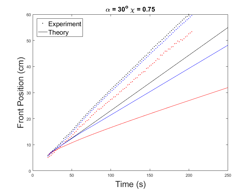
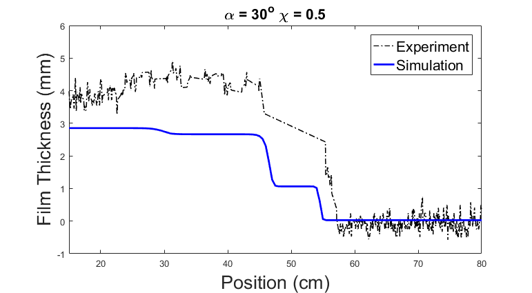
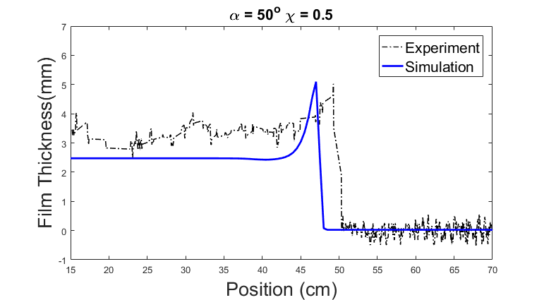
Figures 5 and 6 compare the simulation and experimental results for front position and height profile. In the settled regime, there are three distinct lines in both simulation and experiment corresponding to the three fronts. Although they do not align perfectly, we can see that qualitatively, the fluid and the lighter particles are behaving similarly to simulation, as they are moving with similar velocity. In the ridged regime, the simulated front positions coincide with the experimental results.

In the settled regime, the height profile for the experimental data and theoretical data correspond to each other well, except that the real height is about 1mm higher than predicted. In the ridged regime, again the shape of the graphs from experiment and simulation agrees with each other. But in the simulation, the spike at the slurry front will keep increasing in height as time goes on. This unrealistic behavior depends on the precursor height for the simulation. In this particular example, the precursor height is set to be 1% of the initial height of the slurry. Higher precursor height will prevent this behavior. If the precursor height is set to be 35% or higher, then the front will not keep getting higher forever.
Discussion
We found that the behavior of constant flux bidensity flow is similar to the behavior of constant volume bidensity flow studied in previous work 45. Experimentally, we determine the time required for a regime to emerge, and the critical angle at which the transition between settled and ridged regimes occurs. In addition, we implement a theoretical model that shows the same results. The comparison between the theory and experiment shows good agreement, especially in the ridged regime. Unlike in previous work, the front position grows linearly with time because of the constant flux initial condition.
Future Work
The current model predicts the ridge to grow arbitrarily large in height as time goes on. Further research could look into mitigating this behavior by including a precursor height, i.e. a thickness of the fluid that is already present on the incline before the front reaches it. It may also be useful to look into improving the experimental technique used to measure the height profile to reduce noise. Our model may also be modified to investigate other types of slurries, such as with different size particles.
Acknowledgements
Many thanks to all the undergraduate and graduate students I worked with. In 2016, I worked with Patrick Flynn, Joseph Pappe, William Sisson, Sam Stanton, Jeffrey Wong, Ruiyi Yang. In Spring 2017, I worked with Jessica Bojorquez, Josh Crasto, Dominic Diaz, Margaret Koulikova, Tameez Latib, Andrew Shapiro, and Clover Ye. In Summer 2017, I worked with Jessica Bojorquez, Adam Busis, Chutian Ma, Andrew Shapiro, Qiyao Zhu, and Xinzhe Zuo. My mentors are Dr. David Arnold, Dr. Claudia Falcon, and Dr. Michael Lindstrom. The Principal Investigator (PI) of the lab is Dr. Andrea Bertozzi. Thank you to the Science Research Initiative’s Summer Scholars Research Program for funding in 2016. This material is based upon work supported by the National Science Foundation under grants DMS-1312543, DMS-1659676, and DMS-1045536.
Bibliography
-
Herbert E Huppert. Flow and instability of a viscous current down a slope. Nature, 300(5891):427–429, 1982. ↩︎
-
D. Leighton and A. Acrivos. The shear-induced migration of particles in concentrated suspensions. Journal of Fluid Mechanics, 181:415–439, August 1987. ↩︎
-
N Murisic, J Ho, V Hu, P Latterman, T Koch, K Lin, M Mata, and AL Bertozzi. Particle-laden viscous thin-film flows on an incline: Experiments compared with a theory based on shear-induced migration and particle settling. Physica D: Nonlinear Phenomena, 240(20):1661–1673, 2011. ↩︎
-
Sungyon Lee, Aliki Mavromoustaki, Gilberto Urdaneta, Kaiwen Huang, and Andrea L Bertozzi. Experimental investigation of bidensity slurries on an incline. Granular Matter, 16(2):269-274, 2014. ↩︎
-
Jeffrey T. Wong and Andrea L. Bertozzi. A conservation law model for bidensity suspensions on an incline. Physica D: Nonlinear Phenomena, 330:47–57, 2016. ↩︎